Mia Tarantola

Imports

import pandas as pd
import seaborn as sns
import matplotlib.pyplot as plt

train_url = "https://raw.githubusercontent.com/middlebury-csci-0451/CSCI-0451/main/data/palmer-penguins/train.csv"
train = pd.read_csv(train_url)

from sklearn.preprocessing import LabelEncoder
le = LabelEncoder()
le.fit(train["Species"])

def prepare_data(df):
  df = df.drop(["studyName", "Sample Number", "Individual ID", "Date Egg", "Comments","Region"], axis = 1)
  df = df[df["Sex"] != "."]
  df = df.dropna()
  y = le.transform(df["Species"])
  df = df.drop(["Species"], axis = 1)
  df = pd.get_dummies(df)
  return df, y

X_train, y_train = prepare_data(train)

X_train.head() #looking at data

	Culmen Length (mm)	Culmen Depth (mm)	Flipper Length (mm)	Body Mass (g)	Delta 15 N (o/oo)	Delta 13 C (o/oo)	Island_Biscoe	Island_Dream	Island_Torgersen	Stage_Adult, 1 Egg Stage	Clutch Completion_No	Clutch Completion_Yes	Sex_FEMALE	Sex_MALE
1	45.1	14.5	215.0	5000.0	7.63220	-25.46569	1	0	0	1	0	1	1	0
2	41.4	18.5	202.0	3875.0	9.59462	-25.42621	0	0	1	1	0	1	0	1
3	39.0	18.7	185.0	3650.0	9.22033	-26.03442	0	1	0	1	0	1	0	1
4	50.6	19.4	193.0	3800.0	9.28153	-24.97134	0	1	0	1	1	0	0	1
5	33.1	16.1	178.0	2900.0	9.04218	-26.15775	0	1	0	1	0	1	1	0

y_train.mean()

0.95703125

Introduction

The purpose of this blog post is to practice implemeting machine learning classifiers on real life data! We are looking at the plamer penguins data set collected by Dr. Kristen Gorman. Here we analyze different attributes to use in our species prediction for penguins

Explore

sns.relplot(data = train, x = "Flipper Length (mm)", y = "Culmen Length (mm)", hue = "Species", size = "Body Mass (g)")

<seaborn.axisgrid.FacetGrid at 0x7f780c3ac9d0>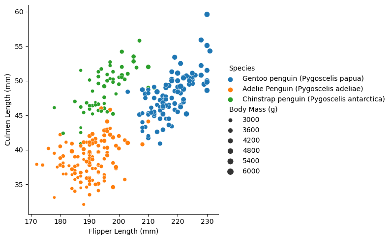

The graph explores the realtionship between species, Flipper Length and Culmen Length. We can see a clear divide between the species. The Gentoo penguins seem to have the longeth flipper and culmen length and are the heaviest. Chinstrap penguins appear to have a longer culmen length but a shorter flipper length. Adelie Penguins have the shortest Flipper and Culmen length. Despite having a longer culmen length, the chinstrap penguins are about the same weight as the Adelies.

train.groupby("Species").agg("mean")

/var/folders/k6/ddn01bfs47n_n5b4t6fb88q80000gp/T/ipykernel_58878/1693257315.py:1: FutureWarning: The default value of numeric_only in DataFrameGroupBy.mean is deprecated. In a future version, numeric_only will default to False. Either specify numeric_only or select only columns which should be valid for the function.
  train.groupby("Species").agg("mean")

	Sample Number	Culmen Length (mm)	Culmen Depth (mm)	Flipper Length (mm)	Body Mass (g)	Delta 15 N (o/oo)	Delta 13 C (o/oo)
Species
Adelie Penguin (Pygoscelis adeliae)	73.440678	38.710256	18.365812	189.965812	3667.094017	8.855229	-25.825165
Chinstrap penguin (Pygoscelis antarctica)	32.696429	48.719643	18.442857	195.464286	3717.857143	9.338671	-24.542886
Gentoo penguin (Pygoscelis papua)	61.930693	47.757000	15.035000	217.650000	5119.500000	8.240438	-26.168937

This tables looks at the quantitative variables averaged by species. It is interesting to see that the Adelie penguins have a deeper culmen, yet are significantly lighter than the Gentoo penguins. In general a larger flipper length correlates to a heavier body mass. However, the penguins with a smaller culmen depth have a lighter body mass.

Picking Attributes and Parameters

First we must check the base rate of our data set - If we were to guess one species for all samples, what would the highest accuracy be? To do this we must calculate the number of each species and compare this to the total number of penguins

num_penguins = y_train.shape[0]
species1 = np.count_nonzero(y_train == 0)
species2 = np.count_nonzero(y_train == 1)
species3 = np.count_nonzero(y_train == 2)

max([species1,species2,species3])/num_penguins

0.4140625

Here we took the spcies with the largest number of samples and divided by the total number of penguins. This gives us our base rate. If we guessed one species for all of the penguins we would be correct at most 41% of the time

Method 1: SVC

from itertools import combinations
import numpy as np
from sklearn.model_selection import train_test_split,GridSearchCV
from sklearn import datasets
from sklearn.svm import SVC
from sklearn.model_selection import cross_val_score

import numpy as np 
# these are not actually all the columns: you'll 
# need to add any of the other ones you want to search for
all_qual_cols = ["Sex","Clutch Completion","Island","Region"]
all_quant_cols = ['Culmen Length (mm)', 'Culmen Depth (mm)', 'Flipper Length (mm)', "Body Mass (g)"]

best_col= []
best_score = -np.inf

best_gamma=np.inf

for qual in all_qual_cols: 
  qual_cols = [col for col in X_train.columns if qual in col ]
  for pair in combinations(all_quant_cols, 2):
    cols = qual_cols + list(pair) 
    for gammas in 10**(np.arange(-4, 4,dtype=float)):
        clf = SVC(gamma = gammas) #kernel="linear",probability=True)
        scores = cross_val_score(clf, X_train[cols], y_train, cv=5)
        if scores.mean()>best_score:
            best_score = scores.mean()
            best_col= cols
            best_gamma = gammas
print(best_col, best_score, best_gamma)

['Island_Biscoe', 'Island_Dream', 'Island_Torgersen', 'Culmen Length (mm)', 'Culmen Depth (mm)'] 0.984389140271493 0.1

The method above chooses the best penguin attributes to use for our model as well as the best gamma, which determines the complexity of the model. To do so we iterate through the different combinations of attributes incluiding 1 qualitative and 2 quantitative variables. We then iterate through a series of gammas and analyze the accuracy of an SVC model using cross validation. The best attributes, score and gamma are recorded for testing

best_model = SVC(gamma = best_gamma)

Here we initialize and train a final model using our initial dataset, and optimized parameters that we just discovered

best_model.fit(X_train[sorted(best_col, reverse = True)],y_train)

SVC(gamma=0.1)

In a Jupyter environment, please rerun this cell to show the HTML representation or trust the notebook.
On GitHub, the HTML representation is unable to render, please try loading this page with nbviewer.org.

test_url = "https://raw.githubusercontent.com/middlebury-csci-0451/CSCI-0451/main/data/palmer-penguins/test.csv"
test = pd.read_csv(test_url)

X_test, y_test = prepare_data(test)
best_model.score(X_test[sorted(best_col,reverse=True)], y_test)

0.9558823529411765

We can see that the final model predicts a penguins species, given their island, culmen length and culmen depth with 95% accuracy. This is definitely better than our base rate, However, we will now experiment with a different method to see if we can increase our results

Method 2 Decision Tree

from itertools import combinations
import numpy as np
from sklearn.tree import DecisionTreeClassifier
from sklearn.model_selection import cross_val_score

import numpy as np 
# these are not actually all the columns: you'll 
# need to add any of the other ones you want to search for
all_qual_cols = ["Sex","Clutch Completion","Island"]
all_quant_cols = ['Culmen Length (mm)', 'Culmen Depth (mm)', 'Flipper Length (mm)', "Body Mass (g)", "Delta 15 N (o/oo)"]

best_col= []
best_score = -np.inf

maximum=np.inf

for qual in all_qual_cols: 
  qual_cols = [col for col in X_train.columns if qual in col ]
  for pair in combinations(all_quant_cols, 2):
    cols = qual_cols + list(pair) 
    for depth in range(2,25):
        clf = DecisionTreeClassifier(max_depth = depth)
        scores = cross_val_score(clf, X_train[cols], y_train, cv=4)
        if scores.mean()>best_score:
            best_score = scores.mean()
            best_col= cols
            maximum = depth
print(best_col, best_score, maximum)

['Island_Biscoe', 'Island_Dream', 'Island_Torgersen', 'Culmen Length (mm)', 'Culmen Depth (mm)'] 0.984375 4

Similar to the method above, we begin by iterating through all combinations of attributes. Next we use cross validation to determine the best value for maximum depth. We keep track of the best attributes, score and depth.

model = DecisionTreeClassifier(max_depth = maximum)
model.fit(X_train[sorted(best_col)],y_train)
model.score(X_test[sorted(best_col)], y_test).round(3)

0.985

We trained a final model with our optimal parameters and tested it our test data. The final model predicted the correct penguin species 98.5% of the time. This is better than the base rate as well as the SVC model. We will now dive further into the accruacy of this model

We will look at a confusion matrix to see what our accuracy loss is originating. As we can see below, the model preformed accrurate on all but one penguin. This penguin was species1 however our model predicted that it was a species 2 penguin.

from sklearn.metrics import confusion_matrix
y_pred = model.predict(X_test[sorted(best_col)])

confusion_matrix(y_test, y_pred)

array([[32,  1,  0],
       [ 0, 12,  0],
       [ 0,  0, 23]])

Visualizing the decision tree classifier

from matplotlib import pyplot as plt
import numpy as np

from matplotlib.patches import Patch

def plot_regions(model, X, y):
    
    x0 = X[X.columns[0]]
    x1 = X[X.columns[1]]
    qual_features = X.columns[2:]
    
    fig, axarr = plt.subplots(1, len(qual_features), figsize = (7, 3))

    # create a grid
    grid_x = np.linspace(x0.min(),x0.max(),501)
    grid_y = np.linspace(x1.min(),x1.max(),501)
    xx, yy = np.meshgrid(grid_x, grid_y)
    
    
    XX = xx.ravel()
    YY = yy.ravel()

    for i in range(len(qual_features)):
      XY = pd.DataFrame({
          X.columns[0] : XX,
          X.columns[1] : YY
      })

      for j in qual_features:
        XY[j] = 0

      XY[qual_features[i]] = 1

      p = model.predict(XY)
      p = p.reshape(xx.shape)
      
      
      # use contour plot to visualize the predictions
      axarr[i].contourf(xx, yy, p, cmap = "jet", alpha = 0.2, vmin = 0, vmax = 2)
      
      ix = X[qual_features[i]] == 1
 
      # plot the data
      axarr[i].scatter(x0[ix], x1[ix], c = y[ix], cmap = "jet", vmin = 0, vmax = 2)
      
      axarr[i].set(xlabel = X.columns[0], 
            ylabel  = X.columns[1])
      
      patches = []
      for color, spec in zip(["red", "green", "blue"], ["Adelie", "Chinstrap", "Gentoo"]):
        patches.append(Patch(color = color, label = spec))

      plt.legend(title = "Species", handles = patches, loc = "best")
      
      plt.tight_layout()


plot_regions(model,X_train[sorted(best_col)],y_train)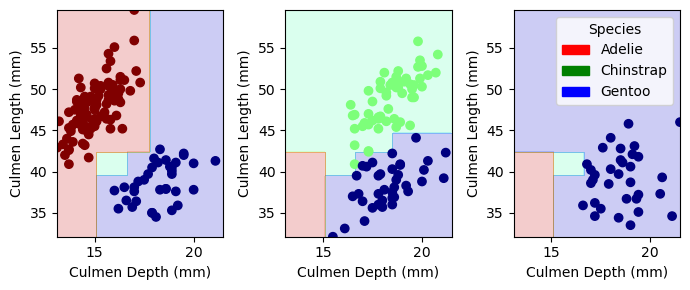

The plots above visualize our decision regions for the decision tree model. We can see that our model does a pretty good job at separating the different species; however, the middle plot has some samples right on the edge

Conclusion

This blog post allowed me to practice a machine learning workflow and get hands on experience implementing a classifier with real data. I really enjoyed exploring the different classification models and optimization parameters. I also enjoyed working with real life data, I can really see how this will help me in my future!