Mia Tarantola Perceptron Blog Post

Introduction

In this blog post we will delve into the perceptron algorithm. I have implemented a algorithm that separates binary data. We have also conducted experiments that push the limits of our algorithm and show cases different patterns

Importing Packages

import pandas as pd
import numpy as np
import seaborn as sns
from matplotlib import pyplot as plt
from sklearn.datasets import make_blobs

#importing perceptron.py code and updating
import perceptron
from perceptron import Perceptron
import importlib
importlib.reload(perceptron)

<module 'perceptron' from '/Users/mtarantola@middlebury.edu/Downloads/Machine Learning/miatarantola.github.io/posts/Perceptron Blog Post/perceptron.py'>

Walk Through of the Update Function

The following function is used to update the perceptron weights:

\(\tilde{w} ^{(t+1)} = \tilde{w} ^ {(t)} + \mathbb{1}(\tilde{y_i} \langle \tilde{w}^{(t)}, \tilde{x_i} \rangle < 0) \tilde{y_i} \tilde{x_i}\)

In order to implement this algorithm, we must follow these steps.

\({1.}\) pick a random index \(~{i} \in\) n.

\({2. }\) predict the label, \(\hat{y_i}\), of our randomly selected data point, \(\tilde{x_i}\).

To do so we calculate the dot product, \(\langle \tilde{w}^{(t)}, \tilde{x_i} \rangle\) and compare the resulting value to 0.

if the result is greater than 0 return 1, otherwise return -1.

\({3.}\) compute \(\mathbb{1}(\tilde{y_i} \langle \tilde{w}^{(t)}, \tilde{x_i} \rangle < 0)\)

Given our predicted label, \(\hat{y_i}\) , of 1 or -1 we can multiply by \(\tilde{y_i}\) to check for correctness

If \(\hat{y_i} \tilde{y_i} <0\) then the signs of our observed and predicted label do not match. If \(\hat{y_i} \tilde{y_i} >0\) then the signs of our predicted and observed label match

So, \(\mathbb{1}(\tilde{y_i} \langle \tilde{w}^{(t)}, \tilde{x_i} \rangle < 0)\) returns 1 if model predicted incorrectly and \(\tilde{y_i} \tilde{x_i}\) is added to the pre-existing weights.

Otherwise the expression returns 0 for a correctly prediction and no update is performed

Experiments

Data that is linearly separable

np.random.seed(8674)

n = 100
p_features = 3

X1, y1 = make_blobs(n_samples = 100, n_features = 2,centers=[(-1.7,-1.7),(1.7,1.7)])

fig1 = plt.scatter(X1[:,0], X1[:,1], c = y1)
xlab = plt.xlabel("Feature 1")
ylab = plt.ylabel("Feature 2")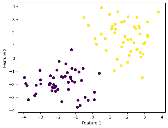

p1 = Perceptron()

p1.fit(X1,y1,100000)

fig1 = plt.plot(p1.history)
xlab = plt.xlabel("Iteration")
ylab = plt.ylabel("Accuracy")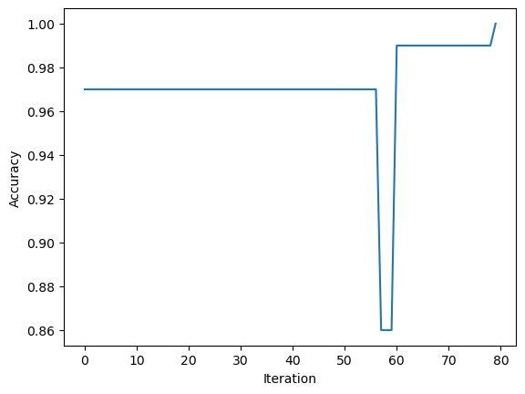

p1.score(X1,y1)

1.0

def draw_line(w, x_min, x_max):
  x = np.linspace(x_min, x_max, 101)
  y = -(w[0]*x + w[2])/w[1]
  plt.plot(x, y, color = "black")

fig = plt.scatter(X1[:,0], X1[:,1], c = y1)
fig = draw_line(p1.w, -2, 2)

xlab = plt.xlabel("Feature 1")
ylab = plt.ylabel("Feature 2")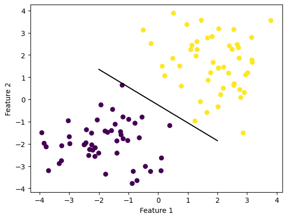

For this experiment we ran our perceptron algorithm on linearly separable data. We can see that the reuslting line is a good separator as it clearly separates our two labels. It is interesting to see that the accuracy decreases before it increases. Another result that suggests our separator is a good fit is that our algorithm stops before the maximum number of iterations allowed

Data that is not linearly separable

np.random.seed(7810) #7810

n = 100
p_features = 3

X2, y2 = make_blobs(n_samples = 100,n_features=2, centers=2)

fig2 = plt.scatter(X2[:,0], X2[:,1], c = y2)
xlab = plt.xlabel("Feature 1")
ylab = plt.ylabel("Feature 2")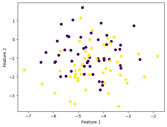

p2 = Perceptron()

p2.fit(X2,y2,1000)

fig3 = plt.plot(p2.history)
xlab = plt.xlabel("Iteration")
ylab = plt.ylabel("Accuracy")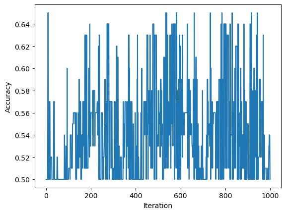

p2.score(X2,y2)

0.5

fig = plt.scatter(X2[:,0], X2[:,1], c = y2)
fig = draw_line(p2.w, -2, 2)

xlab = plt.xlabel("Feature 1")
ylab = plt.ylabel("Feature 2")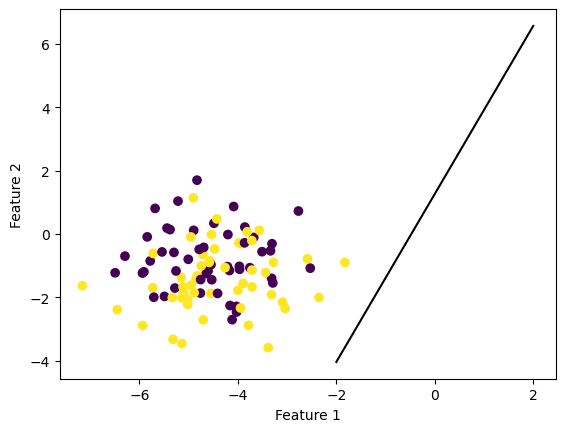

This experiment displays the use of our perceptron algorithm on nonlinearly separable data. As shown above, the resulting line is not a good separater. In fact, it isn’t separating any data. We can also see the inaccuracy by tracking the accuracy over iterations. We can see that the algorihtm is not converging to one set of weights and thus has not found an optimizer.

The perceptron algorithm in >2 dimensions

np.random.seed(7810) #7810

n = 100

X3, y3 = make_blobs(n_samples = 100,n_features=6, centers=2)

p3 = Perceptron()

p3.fit(X3,y3,1000)

fig4 = plt.plot(p3.history)
xlab = plt.xlabel("Iteration")
ylab = plt.ylabel("Accuracy")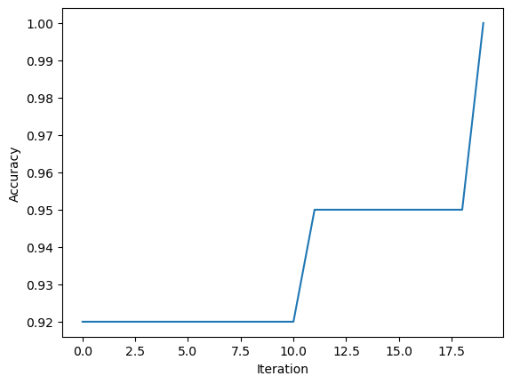

p3.score(X3,y3)

1.0

Yes, I do believe that my data is linearly separable because my perceptron’s accuracy converges to 1 after 18 iterations. This means that my perceptron reached 100% accuracy and did not complete upon reaching that maximum number of iterations.

Ending Question

The time complexity for a single iteration of the perceptron algorithm is O(p) because predicting the label of a single data point requires calculating the dot product of x and w. Thus, np iterates over the p features of x to calulate the dot product. All other steps of this equation invlove simple multiplication or addition which are O(1).